How to change the coordinate system of annotations in Matplotlib

When adding annotations in matplotlib, you might want to change the coordinate system to use: relative to the figure, using the data coordinates, or others.

There are actually a large number of possibilities, so you can choose the one that best fits your needs.

This post explains step-by-step everything you need to understand to change and manipulate the coordinate system in matplotlib.

Libraries

For creating this chart, we will need to load the following libraries:

matplotlib for creatin the chart

import matplotlib.pyplot as plt

# set a higher resolution
plt.rcParams['figure.dpi'] = 200

Coordinates

Matplotlib provides a way to change and specify which coordinates system to use with exhaustive possibilites:

the figure?
the axes?
the data?
other?

In order to change the coordinate system, you have to change the transform argument of the text() function. Here are the possibilities:

ax.transData: the data coordinates
ax.transAxes: the axes coordinates
fig.transFigure: the figure coordinates
fig.dpi_scale_trans: physical coordinates
and others that we will see in the following examples.

import matplotlib.pyplot as plt
from matplotlib.transforms import IdentityTransform

fig, ax = plt.subplots(figsize=(10, 10))
ax.plot([0, 3], [30, 10], color='#d9f1fa')

# Data coordinates (default)
ax.text(
   2, 20,
   'Data coords\nx=2, y=20\ntransformax.transData',
   color='blue',
   fontweight='bold', fontsize=14)

# Axes coordinates
ax.text(
   0.5, 0.1,
   'Axes coords\nx=0.5, y=0.1\ntransform=ax.transAxes',
   transform=ax.transAxes,
   color='green',
   fontweight='bold', fontsize=14)

# Figure coordinates
ax.text(
   0.5, 0.9,
   'Figure coords\nx=0.5, y=0.9\ntransform=fig.transFigure',
   transform=fig.transFigure,
   color='red',
   fontweight='bold', fontsize=14)

# Blended transformation
trans = ax.get_xaxis_transform()  # x in data, y in axes
ax.text(
   2, 0.8,
   'Blended coords\nx=2, y=0.8\ntransform=ax.get_xaxis_transfor()',
   transform=trans,
   color='purple',
   fontweight='bold', fontsize=14)

# Inches coordinates
ax.text(
   2, 5,
   'Inches coords\nx=2, y=5\ntransform=fig.dpi_scale_trans',
   transform=fig.dpi_scale_trans,
   color='orange',
   fontweight='bold', fontsize=14)

plt.show()

Don't worry if this is confusing, we will go over each of these cases in the following sections.

Quick reminder on figure and axes

In Matplotlib, the figure is the top-level container that holds all the elements of the chart. It is the canvas on which the chart is drawn. The axes are the actual plot. They are the region of the figure where the data is plotted.

One figure can contains one or multiple axes. In the case of multiple axes, they can be arranged in a grid, like in a subplot.

Here is an example of a figure with 2 (empty) axes:

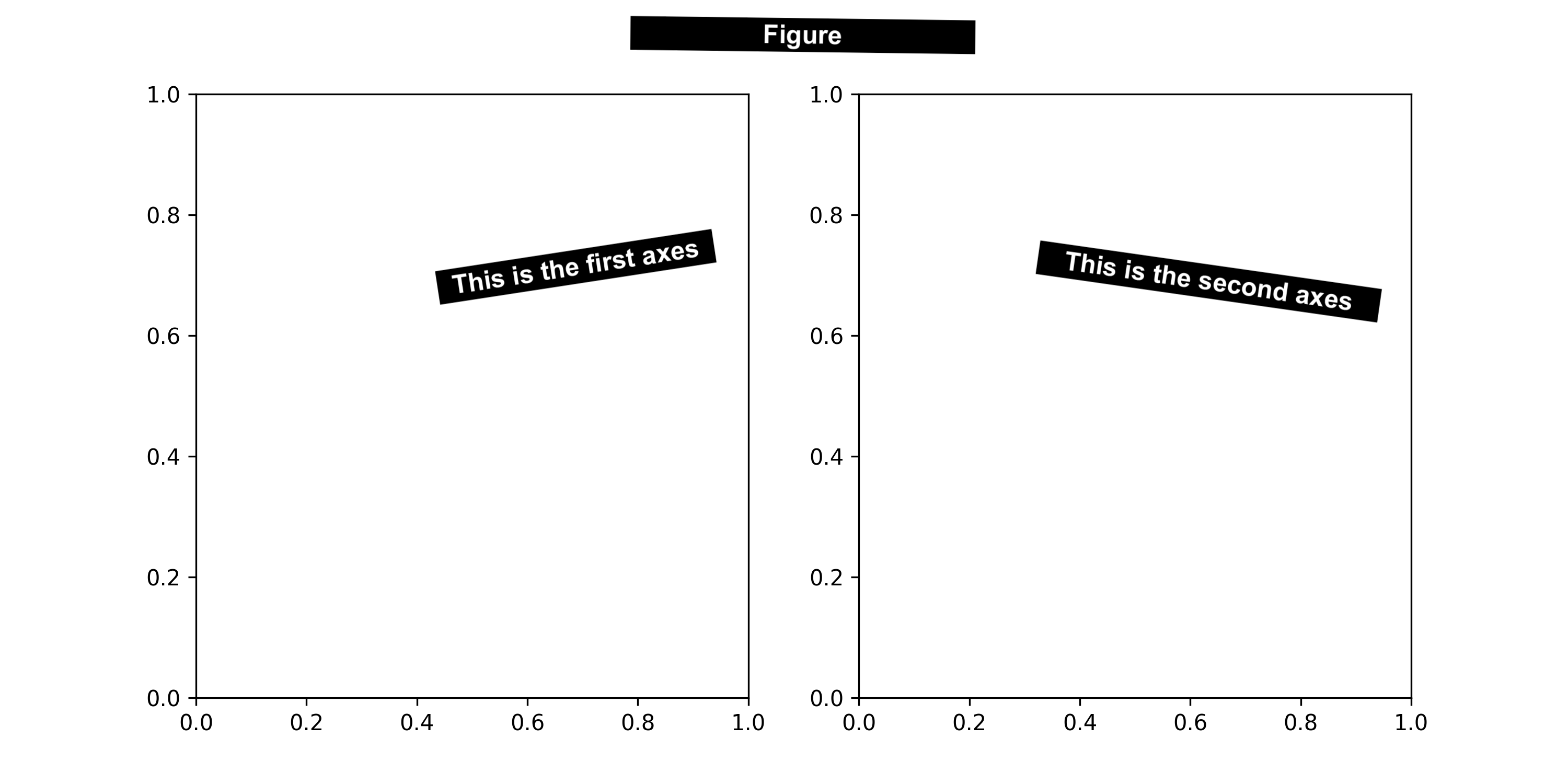
Reproduce it with:

fig, ax = plt.subplots(nrows=1, ncols=2, figsize=(10, 5))
plt.show()

Data coordinates: `ax.transData`

The data coordinate system is the one that is used to plot the data. For example, if you create a scatter plot with x=[1,2,3] and y=[4,5,6], the data coordinate system will be the one that goes from 1 to 3 on the x-axis and from 4 to 6 on the y-axis.

It's the default coordinate system used by Matplotlib when you plot data. You can access it with ax.transData. Let's see an example:

Note: we specify transform=ax.transData but since it's the default one, you can omit it.

x = [1, 2, 3]
y = [4, 5, 6]

fig, ax = plt.subplots()
ax.plot(x, y)

# Data coordinates
ax.text(
   x=1, y=5.5,
   s='x=1, y=5.5\ntransform=ax.transData',
   transform=ax.transData,
   fontsize=12
)

plt.show()

Axes coordinates: `ax.transAxes`

The axes coordinate system is the one that goes from 0 to 1 on each axis.

In this case, the positions will be relative to the axes: (0,0) is the bottom-left corner of the axes, and (1,1) is the top-right corner.

x = [1, 2, 3]
y = [4, 5, 6]

fig, ax = plt.subplots(ncols=2, figsize=(10, 5))
ax[0].plot(x, y)
ax[1].plot(y, x)

# Axes coordinates for left subplot
ax[0].text(
   x=0.1, y=0.8,
   s='x=0.1, y=0.8\ntransform=ax.transAxes',
   transform=ax[0].transAxes,
   fontsize=10,
)

# Axes coordinates for right subplot
ax[1].text(
   x=0.15, y=0.6,
   s='x=0.15, y=0.6\ntransform=ax.transAxes',
   transform=ax[1].transAxes,
   fontsize=10,
)

plt.show()

Figure coordinates: `fig.transFigure`

The figure coordinate system spans from 0 to 1 across the entire figure. This is the most intuitive system: the bottom left corner is (0,0), and the top right corner is (1,1).

It is particularly useful for adding annotations that are absolute to the figure, such as a title or credit.

An even cooler feature is that you can specify values above 1 and below 0. For instance, to add a title slightly above the figure's top, you can use (0.5, 1.1) for the position.

Note: The primary difference between ax.text() and fig.text() lies in the coordinate system used, meaning the following are equivalent:

fig, ax = plt.subplots()

# This line
ax.text(0.5, 0.5, 'text', transform=fig.transFigure)

# Is equivalent to this one
fig.text(0.5, 0.5, 'text')

x = [1, 2, 3]
y = [4, 5, 6]

fig, ax = plt.subplots(ncols=2, figsize=(10, 5))
ax[0].plot(x, y)
ax[1].plot(y, x)

# Figure coordinates
ax[0].text(
   x=0.15, y=0.7,
   s='x=0.15, y=0.7\ntransform=fig.transFigure',
   transform=fig.transFigure,
   fontsize=10,
)

# This is equivalent to the previous one: it will be displayed in the same position
ax[1].text(
   x=0.15, y=0.7,
   s='x=0.15, y=0.7\ntransform=fig.transFigure',
   transform=fig.transFigure,
   fontsize=10,
)

plt.show()

Relative to x-axis and to y-axis

Thanks to the ax.get_xaxis_transform() and ax.get_yaxis_transform() functions, you can specify a position relative to the x-axis or the y-axis while the other coordinate is in data coordinates.

x = [1, 2, 3]
y = [4, 5, 6]

fig, ax = plt.subplots(ncols=2, figsize=(10, 5))
ax[0].plot(x, y)
ax[1].plot(y, x)

# Semi-blended transformation: x in data coordinates, y in axes coordinates
ax[0].text(
   x=1, y=0.8,
   s='x=1, y=0.8\ntransform=ax.get_xaxis_transform()',
   transform=ax[0].get_xaxis_transform(),
   fontsize=10,
)

# Semi-blended transformation: y in data coordinates, x in axes coordinates
ax[1].text(
   x=0.15, y=2,
   s='x=0.15, y=2\ntransform=ax.get_yaxis_transform()',
   transform=ax[1].get_yaxis_transform(),
   fontsize=10,
)

plt.show()

Physical coordinates: `fig.dpi_scale_trans`

Sometimes we want an object to be a certain physical size on the plot: for example, a circle of 1cm radius. This is what the fig.dpi_scale_trans is for. It allows you to specify the size of an object in inches.

x = [1, 2, 3]
y = [4, 5, 6]

fig, ax = plt.subplots(figsize=(8, 5))
ax.plot(x, y)

# Position in inches from the lower-left (x=0,y=0) corner of the figure
ax.text(
   x=1, y=3,
   s='x=1, y=3\ntransform=fig.dpi_scale_trans',
   transform=fig.dpi_scale_trans,
   fontsize=10,
)

plt.show()

Going further

Contact & Edit

👋 This document is a work by Yan Holtz. You can contribute on github, send me a feedback on twitter or subscribe to the newsletter to know when new examples are published! 🔥

This page is just a jupyter notebook, you can edit it here. Please help me making this website better 🙏!

How to change the coordinate system of annotations in Matplotlib

Libraries

Coordinates

Quick reminder on figure and axes

Data coordinates: ax.transData

Axes coordinates: ax.transAxes

Figure coordinates: fig.transFigure