Faceted scatterplot with regression seaborn

Libraries

First, we need to load a few libraries:

seaborn: for creating the scatterplot
matplotlib: for displaying the plot
pandas: for data manipulation

import pandas as pd
import matplotlib.pyplot as plt
import seaborn as sns

sns.set_style("darkgrid")

Dataset

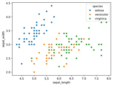
Since scatter plot are made for visualizing relationships between two numerical variables, we need a dataset that contains at least two numerical columns.

Here, we will use the iris dataset that we load directly from the gallery:

path = 'https://raw.githubusercontent.com/holtzy/The-Python-Graph-Gallery/master/static/data/iris.csv'
df = pd.read_csv(path)
df.head()

	sepal_length	sepal_width	petal_length	petal_width	species
0	5.1	3.5	1.4	0.2	setosa
1	4.9	3.0	1.4	0.2	setosa
2	4.7	3.2	1.3	0.2	setosa
3	4.6	3.1	1.5	0.2	setosa
4	5.0	3.6	1.4	0.2	setosa

Simple splitting with a categorical variable

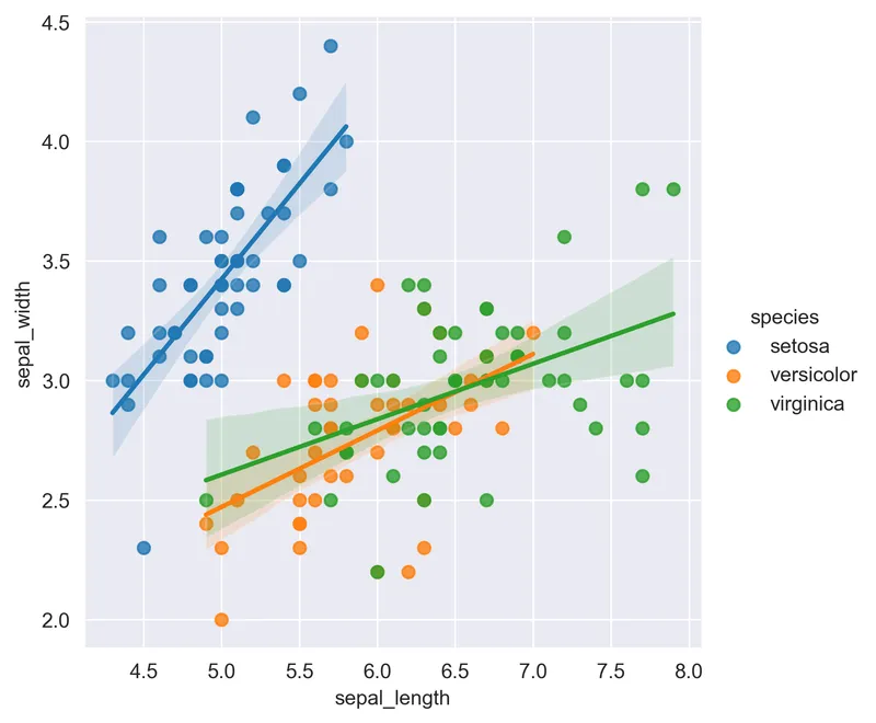
The lmplot() function requires the following 4 arguments to create a faceted scatterplot:

x : column of the variable for the x axis
y: column of the variable for the y axis
hue: column of the variable for the facet.
data : data frame with all columns

Faceted scatterplot with regression seaborn: Simple splitting with a categorical variable

sns.lmplot(
    x="sepal_length",
    y="sepal_width",
    data=df,
    hue="species",
)
plt.show()

Multiple subplots

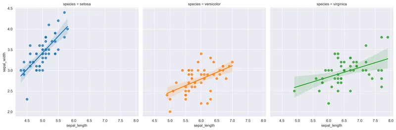
You can also use the col argument and assign it the same value as the hue to create subplots instead of a single one:

Faceted scatterplot with regression seaborn: Multiple subplots

sns.lmplot(
    x="sepal_length",
    y="sepal_width",
    data=df,
    hue="species",
    col="species"
)
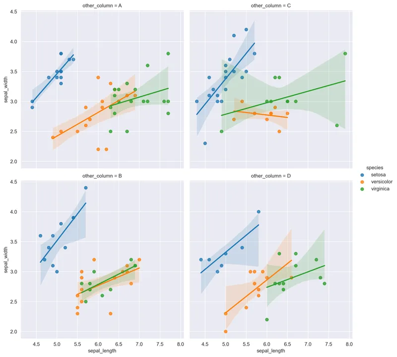
plt.show()

Split with a 4th column

You can also custom the line width and style with the linewidth and linestyle values:

Faceted scatterplot with regression seaborn: Split with a 4th column

import numpy as np
df["other_column"] = np.random.choice(['A', 'B', 'C', 'D'], size=len(df))

sns.lmplot(
    x="sepal_length",
    y="sepal_width",
    data=df,
    hue="species",
    col="other_column",
    col_wrap=2 # maximum of 2 columns
)
plt.show()

Going further

This post explains how to customize the appearance of a regression fit in a scatter plot with seaborn.

You might be interested in more advanced examples on: