Basic Connected Scatterplot for Evolution of Variables

Libraries

First, we need to load a few libraries:

matplotlib: for creating the chart
pandas: for data manipulation

import pandas as pd
import matplotlib.pyplot as plt

Dataset

Our dataset is about the number of people having a certain name, and the evolution of this number over the years. Let's load it with pandas:

# import dataset
df = pd.read_csv("https://raw.githubusercontent.com/holtzy/data_to_viz/master/Example_dataset/5_OneCatSevNumOrdered.csv")
df.head()

	year	sex	name	n	prop
0	1880	F	Helen	636	0.006516
1	1880	F	Amanda	241	0.002469
2	1880	F	Betty	117	0.001199
3	1880	F	Dorothy	112	0.001147
4	1880	F	Linda	27	0.000277

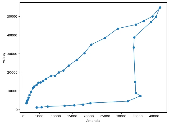
Our goal here is to explore the evolution of the number of people named "Ashley" and "Amanda" over the years in a single scatter plot.

For this, we need to change a bit the dataset:

filter on those 2 names
filter on only date after 1970
pivot the table to have the names as columns and the years as rows, using the pivot_table() function

# filter data
df = df.loc[(df.name=="Ashley") | (df.name=="Amanda")]
df = df.loc[(df.sex=="F") & (df.year>1970)]
df = pd.pivot_table(df, values='n', index=['year'], columns=['name'])

df.head()

name	Amanda	Ashley
year
1971	4133.0	1164.0
1972	4181.0	1176.0
1973	5627.0	1253.0
1974	7476.0	1626.0
1975	12653.0	1988.0

Connected scatterplot for evolution

In practice, we just have to call the plot() function with our columns as arguments. We specify that markers have to be used with marker='o' and that the lines have to be connected with linestyle='-'.

Basic Connected Scatterplot for Evolution of Variables: Connected scatterplot for evolution

fig, ax = plt.subplots(figsize=(8, 6))

# plot the connected scatterplot
ax.plot(df.Amanda, df.Ashley, linestyle='-', marker='o')

# x axis label
plt.xlabel('Amanda')

# y axis label
plt.ylabel('Ashley')

# show the graph
plt.show()

Annotations

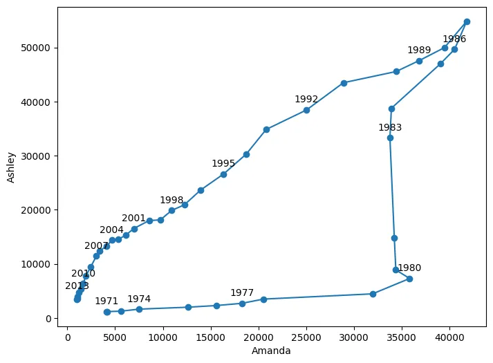
Our last chart has a major issue: we don't know which year is represented by each point.

To fix this, we can use the annotate() function to add a text next to each point. However, it's not necessary to add all the years, and decide to only plot 1 out of 3 years.

In practice, we loop over the number of rows with a step of 3 (thanks to range(0, len(df), 3)) and add an annotation with the annotate() function.

Basic Connected Scatterplot for Evolution of Variables: Annotations

fig, ax = plt.subplots(figsize=(8, 6))

# plot the connected scatterplot
ax.plot(df.Amanda, df.Ashley, linestyle='-', marker='o')

# add annotations in every 3 data points with a loop
for line in range(0, df.shape[0], 3):
     ax.annotate(
          df.index[line], 
          (df.Amanda.iloc[line], df.Ashley.iloc[line]+1000) ,
          va='bottom',
          ha='center'
     )

# labels and display
plt.xlabel('Amanda')
plt.ylabel('Ashley')
plt.show()

What a nice way to visualize the evolution of the number of people named Ashley and Amanda over the years!

Going further

This post explains how to create a connected scatterplot with matplotlib.

You might be interested in how to reproduce this beautiful connected scatter plot and how to create multiple connected scatter plots on the same chart.