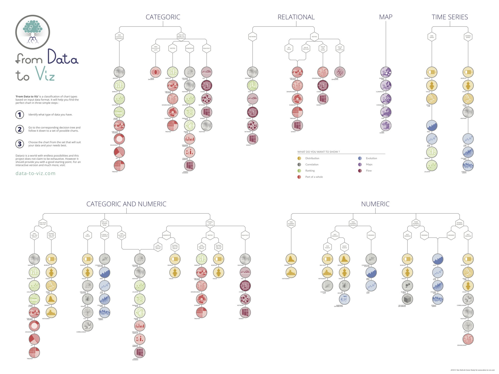
A marginal plot allows to study the relationship between 2 numeric variables. The central chart displays their correlation. It is usually a scatterplot, a hexbin plot, a 2D histogram or a 2D density plot. The marginal charts, usually on the top and right, show the distribution of 2 variables using histogram or density plot.
The seaborn library provides a joint plot function that is really handy to make this type of graphics. The top graph shows its default behaviour, and here are few possible customizations. Seaborn has a nice documentation and some of these examples taken from there.
Central Plot
Seaborn library have jointplot() function to draw a marginal plot. The kind of the central plot can be given as a parameter in jointplot() function:
kind: the possible options are “scatter” | “kde” | “hist” | “hex” | “reg” | “resid”
In this example three marginal plots built with different central plots; scatterplot, hexbin and density.
# library & dataset
import seaborn as sns
import matplotlib.pyplot as plt
df = sns.load_dataset('iris')

# Custom the inside plot: options are: “scatter” | “reg” | “resid” | “kde” | “hex”
sns.jointplot(x=df["sepal_length"], y=df["sepal_width"], kind='scatter')
sns.jointplot(x=df["sepal_length"], y=df["sepal_width"], kind='hex')
sns.jointplot(x=df["sepal_length"], y=df["sepal_width"], kind='kde')

plt.show()
# Then you can pass arguments to each type:
sns.jointplot(x=df["sepal_length"], y=df["sepal_width"], kind='scatter', s=200, color='m', edgecolor="skyblue", linewidth=2)
# Custom the color
sns.set_theme(style="white", color_codes=True)
sns.jointplot(x=df["sepal_length"], y=df["sepal_width"], kind='kde', color="skyblue")
plt.show()Marginal
You can customize the marginal plots with marginal_kws parameter.
# library & dataset
import seaborn as sns
import matplotlib.pyplot as plt
df = sns.load_dataset('iris')

# Custom the histogram:
sns.jointplot(x=df["sepal_length"], y=df["sepal_width"], kind='hex', marginal_kws=dict(bins=30, fill=True))

plt.show()
Ratio
It is also possible to change the central plot-margin plats ratio and the space between the joint and marginal axes.
space: space between the joint and marginal axesratio: ratio of joint axes height to marginal axes height
# library & dataset
import seaborn as sns
import matplotlib.pyplot as plt
df = sns.load_dataset('iris')

# No space
sns.jointplot(x=df["sepal_length"], y=df["sepal_width"], kind='kde', color="grey", space=0)

# Huge space
sns.jointplot(x=df["sepal_length"], y=df["sepal_width"], kind='kde', color="grey", space=3)

# Make marginal bigger:
sns.jointplot(x=df["sepal_length"], y=df["sepal_width"], kind='kde',ratio=1)

plt.show()


