Libraries
First, we need to import a few libraries:
- matplotlib: for plotting
- seaborn: for making the plots prettier
import matplotlib.pyplot as plt
import seaborn as sns
Dataset
The dataset that we will use is the iris dataset that we can load using seaborn.
df = sns.load_dataset('iris')Defaut density plot
Density plot differ from histogram in that they are smoothed versions of the histogram.
However, in order to be smoothed, we need to define a bandwidth, which is a parameter that controls the smoothness of the density plot. Varying the bandwidth will give different density plots, and different information too!
In seaborn, it's the bw_method argument that controls it. Here is what the default bandwidth looks like in seaborn:
sns.set_theme(style="darkgrid")
sns.kdeplot(df['sepal_width'], fill=True, color="olive", bw_method=1)
plt.show()
Custom bandwidth
The following density plots have been made using the same data. Only the bandwidth value changes from 1 in the first graph to 0.2 on the right.
This parameter can be of particular interest when a finer understanding of the distribution is needed. It could highlight bimodal distributions more easily and help us in observing patterns that the Gaussian kernel over-smoothed.
Deprecation:
Note that in older version of seaborn (< 0.11.0), the bw parameter was used but is deprecated since and bw_method and bw_adjust have replaced it.
See scipy.stats.gaussian_kde in scipy.org for further details on bw_method and bw_value.
In seaborn 0.11.0 and before versions, you would use sns.kdeplot(df\['sepal_width'\], shade=True, bw=0.05, color='olive')
Now, shade and bw arguments are deprecated.
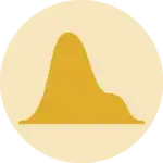
sns.set_theme(style="darkgrid")
sns.kdeplot(df['sepal_width'], fill=True, color='olive', bw_method=0.08)
plt.show()
Going further
This post explains how to control smoothing in a density plot with seaborn.
You might be interested in displaying distribution of multiple variables and creating a mirrored density plot.