Bubble map with Python and Basemap

Libraries

First, we need to load a few libraries:

matplotlib: for basic plotting
pandas: for data manipulation
mpl_toolkits for the Basemap module (maps)

from mpl_toolkits.basemap import Basemap
import matplotlib.pyplot as plt
import pandas as pd

Dataset

Let's load a dataset with geographical information (latitude and longitude columns):

data = pd.read_csv('https://raw.githubusercontent.com/holtzy/The-Python-Graph-Gallery/master/static/data/TweetSurfData.csv', sep=";")
data.head()

	homelon	homelat	homecontinent	n
0	-178.12	-14.29	Australia	10
1	-172.10	-13.76	NaN	2
2	-159.72	21.97	NaN	6
3	-159.59	21.91	North America	4
4	-159.53	22.10	North America	37

Background map

Let's start by building the background map of our bubble map thanks to the basemap library. The basemap library allows to load the boundaries of any region of the world without having to load a shapefile or a geojson file.

You can read more about this step in the map section of the gallery.

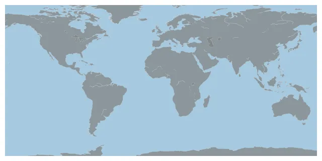
Bubble map with Python and Basemap: Background map

# Initialize the background map
plt.figure(figsize=(8, 10))
m=Basemap(llcrnrlon=-160, llcrnrlat=-75,urcrnrlon=160,urcrnrlat=80)

# Draw boundaries, continents and coastlins
m.drawmapboundary(fill_color='#A6CAE0', linewidth=0)
m.fillcontinents(color='grey', alpha=0.7, lake_color='grey')
m.drawcoastlines(linewidth=0.1, color="white")

# show
plt.show()

Add markers

Bubble map with Python and Basemap: Add markers

# Initialize the background map
plt.figure(figsize=(8, 10))
m=Basemap(llcrnrlon=-160, llcrnrlat=-75,urcrnrlon=160,urcrnrlat=80)

# Draw boundaries, continents and coastlins
m.drawmapboundary(fill_color='#A6CAE0', linewidth=0)
m.fillcontinents(color='grey', alpha=0.7, lake_color='grey')
m.drawcoastlines(linewidth=0.1, color="white")

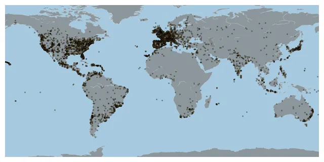
# Add a point per position
m.scatter(
    data["homelon"],
    data["homelat"],
    alpha=0.4,
    s=1,
    c="orange",
    linewidth=1,
    edgecolor="black"
)

# show
plt.show()

Bubble size

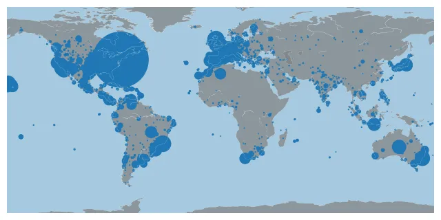
It can be interesting to use the size of the bubble to represent a 3rd variable. In this case, the size of the bubble is proportional to the n in the dataset.

You can control the size of the bubble by changing the s argument of the scatter() function.

Bubble map with Python and Basemap: Bubble size

# Initialize the background map
plt.figure(figsize=(8, 10))
m=Basemap(llcrnrlon=-160, llcrnrlat=-75,urcrnrlon=160,urcrnrlat=80)

# Draw boundaries, continents and coastlins
m.drawmapboundary(fill_color='#A6CAE0', linewidth=0)
m.fillcontinents(color='grey', alpha=0.7, lake_color='grey')
m.drawcoastlines(linewidth=0.1, color="white")

# Add a point per position
m.scatter(
    data["homelon"],
    data["homelat"],
    s=data["n"]/10
)

# show
plt.show()

Custom bubble style

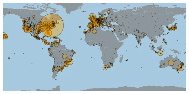
For better looking map, we can customize the bubble style with the following arguments:

alpha: transparency of the bubble
edgecolor: color of the bubble border
linewidth: width of the bubble border
c: color of the bubble

Bubble map with Python and Basemap: Custom bubble style

# Initialize the background map
plt.figure(figsize=(8, 10))
m=Basemap(llcrnrlon=-160, llcrnrlat=-75,urcrnrlon=160,urcrnrlat=80)

# Draw boundaries, continents and coastlins
m.drawmapboundary(fill_color='#A6CAE0', linewidth=0)
m.fillcontinents(color='grey', alpha=0.7, lake_color='grey')
m.drawcoastlines(linewidth=0.1, color="white")

# Add a point per position
m.scatter(
    data["homelon"],
    data["homelat"],
    alpha=0.4,
    s=data["n"]/10,
    c="orange",
    linewidth=1,
    edgecolor="black"
)

# show
plt.show()

Going further

This post explains how to create and custom a bubble map with Python.

If you want to go further, you can also create a choropleth map or a connection map with Python.